Beim "klassischen"
Diffusions-Quanten-Monte-Carlo-Verfahren wird die Potenzialhyperfläche mit einer
Schar von "Random-Walkers" abgetastet. Die Wellenfunktion ergibt sich dann aus
der Häufigkeit der Walker-Positionen.Ein Beispiel (H2-Molekül)
hierfür findet man hier.
Im folgenden Programm wird eine
Trial-Wellenfunktion mit den Elektronen als Walker abgetastet. Die potenzielle
Energie wird als Mittelwert über die Walker-Positionen bestimmt. Daraus kann mit
Hilfe des Virialtheorems die Gesamtenergie bestimmt werden. Das Verfahren hat
den Vorteil, dass man die Bewegung der Elektronen anschaulich darstellen und
dass man mit einem analytischen Ausdruck für die Wellenfunktion experimentieren
kann.
Quantum-Monte-Carlo für das Heliumatom unter Verwendung der Bibliotheken JSci (A Science API for Java, http://sourceforge.net/projects/jsci/) und OSP (OpenSourcePhysics, www.opensourcephysics.org/) als Ausgangsbasis. JSci liefert 3DVektoren, OSP eine komfortable grafische Darstellung. Für jede Teilchen-Koordinate wird ein Walker verwendet (kein Entstehen und Vergehen von Walkern). Das Programm kann leicht auf andere Systeme erweitert werden und man kann damit experimentieren (Variation der Anzahl der Schritte, der Schrittweite, der Wellenfunktion). Beispiele: H, Li, H2.
Diese Seite kann auch als pdf-Datei heruntergeladen werden, Source-Code als jGRASP-Projekt.
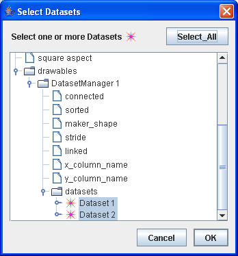
Mit jGRASP:
mit n = 40 in Befehlszeile (Run Arguments)
|
Run main:
 |
Mit Views/Scale
|
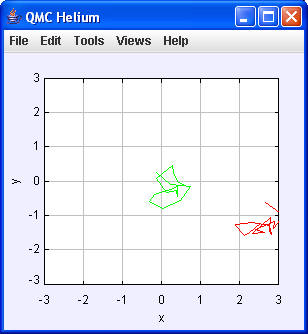 |
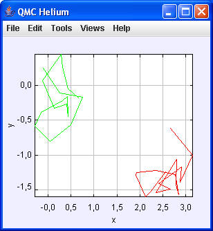
Über Tools/DatasetTool kann man die Darstellung weiter variieren
 |
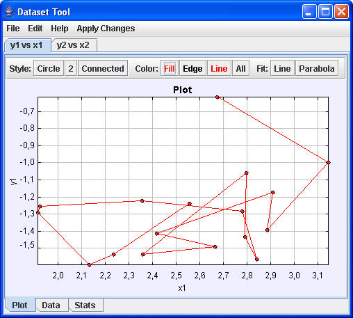 |
Die Daten kann man sich auch als Tabelle ausgeben lassen:
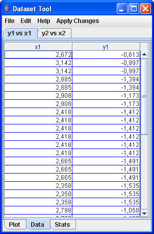 |
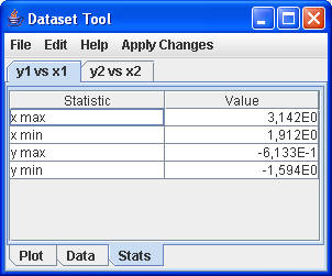 |
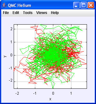
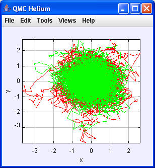
Mit einer größeren Anzahl von Walker-Schritten wird die Elektronen-Verteilung deutlicher:
| N = 2000
|
N = 20000
|
Kommentierter Source-Code
Die blau-grau hervorgehobenen Passagen sind aus OSP eingefügt. Eigene Kommentare sind hell-grün hervorgehoben.
MonteCarlo.java
import java.io.*;
import JSci.maths.*;
import JSci.maths.statistics.*;
import JSci.io.*;
import java.awt.Color;
import
org.opensourcephysics.frames.PlotFrame;
import org.opensourcephysics.display.*;
/**
* Monte Carlo calculation of Helium ground state energy.
* @author Mark Hale
* @version 1.0
*/
public final class MonteCarlo implements Mapping
{
private int N; //
walker steps
private double energy[];
// 1D array of local energy
private DoubleVector r1;
// radius vector of electron1
private DoubleVector r2;
PlotFrame frame = new PlotFrame("x", "y", "QMC
Helium"); // (String xlabel, String ylabel, String frameTitle)
/**
* Instantiate class.
*/
public static void main(String arg[])
{
if(arg.length==1)
{
int n=Integer.valueOf(arg[0]).intValue();
// for command line input
new MonteCarlo(n);
}
else
{
System.out.println("Need to specify command
line arguments:");
System.out.println("<number of iterations>");
}
}
/**
* Constructor.
* @param n number of iterations
*/
public MonteCarlo(int n)
{
N=n; //
walker steps
r1=new Double3Vector(Math.random(),Math.random(),Math.random());
// components x1, y1, z1 with random
numbers
// between 0 and 1 as initial walker
position
r2=new Double3Vector(-Math.random(),-Math.random(),-Math.random());
// same for electron2 but with opposite
// sign
energy=new double[N];
frame.setConnected(0, true);
// Points are connected by straight lines
frame.setMarkerShape(0, Dataset.NO_MARKER);
// Shapes are: NO_MARKER, CIRCLE, SQUARE, AREA, PIXEL, BAR, POST
// weitere Methoden: setMarkerSize(int datasetIndex, int markerSize)
// setMarkerColor(int datasetIndex, Color color)
frame.setConnected(1, true);
frame.setMarkerShape(1, Dataset.NO_MARKER);
frame.setVisible(true);
compute();
saveResults();
frame.setDefaultCloseOperation(javax.swing.JFrame.EXIT_ON_CLOSE);
frame.setXPointsLinked(true);
// default is true
// X data for datasets > 0 will not be shown in a table
view
frame.setXYColumnNames(0,"x1","y1");
// Sets the column names when rendering this dataset in a JTable
frame.setXYColumnNames(1,"x2","y2");
frame.setRowNumberVisible(true);
// Table displays row number
}
/**
* Compute the ground state energy.
*/
private void compute()
{
DoubleVector tmpr1,tmpr2;
double prob,tmpprob;
// Stabilising
for(int i=0;i<1000;i++)
{
tmpr1=r1.mapComponents(this);
// mapComponents() applies a function on
all vector components, here a new walker step
// (->
map())
tmpr2=r2.mapComponents(this);
tmpprob=trialWF(tmpr1,tmpr2);
// applies the trial wave function on
the new coordinates of the two electrons
tmpprob*=tmpprob;
prob=trialWF(r1,r2);
// applies the trial wave function on
the old coordinates of the two electrons
prob*=prob;
if(tmpprob/prob>Math.random())
// now it depends on this condition
whether the new coordinates will be accepted
{
r1=tmpr1;
r2=tmpr2;
}
}
System.out.println("Integrating...");
System.out.println("r1 in
Stabilising: " + r1); // for
monitoring only
System.out.println("x1 mit r1.getComponent(0): " +
r1.getComponent(0));
for(int i=0;i<N;i++)
// here the actual walk begins
{
tmpr1=r1.mapComponents(this);
tmpr2=r2.mapComponents(this);
tmpprob=trialWF(tmpr1,tmpr2);
tmpprob*=tmpprob;
prob=trialWF(r1,r2);
prob*=prob;
if(tmpprob/prob>Math.random())
{
r1=tmpr1;
r2=tmpr2;
}
energy[i]=localEnergy(r1,r2);
//System.out.println("r1
= " + r1); // for
monitoring purposes
//System.out.println("r2 = " + r2);
//System.out.println("energy[ " + i + " ] =
" + energy[i]);
frame.append(0, r1.getComponent(0), r1.getComponent(1));
// append(int datasetIndex, double x, double y)
frame.append(1, r2.getComponent(0), r2.getComponent(1));
frame.setVisible(true);
frame.repaint();
// Damit wird Grafik laufend
dargestellt, was sehr rechenintensiv ist!
}
}
/**
* Trial wavefunction.
* @param r1 position vector of electron 1
* @param r2 position vector of electron 2
*/
private double trialWF(DoubleVector
r1,DoubleVector r2)
{
double modR1=r1.norm();
// square root of (x^2 + y^2 +z^2)
double modR2=r2.norm();
double modR12=r1.subtract(r2).norm();
// sqrt of ( (x1^2-x2^2) + ...)
return Math.exp(-2*modR1)*Math.exp(-2*modR2)*Math.exp(modR12/2);
// general formula of a two-electron
system
}
/**
* Local energy calculation.
* @param r1 position vector of electron 1
* @param r2 position vector of electron 2
*/
private double localEnergy(DoubleVector
r1,DoubleVector r2)
{
DoubleVector r12=r2.subtract(r1);
double
termR112=r1.scalarProduct(r12)/(r1.norm()*r12.norm());
double
termR212=r2.scalarProduct(r12)/(r2.norm()*r12.norm());
return -17/4-termR112+termR212;
// expression for local energy
}
/**
* Update electron co-ordinates.
*/
public double map(double x)
{
return x+(Math.random()-0.5);
// random walk steps between -0.5 and
+0.5
}
/**
* Not used, dummy implementation for Mapping interface.
*/
public Complex map(Complex z)
{
return null;
}
/**
* Log results to disk.
*/
private void saveResults()
{
File file=new File("results.dat");
char buf[]=null;
NormalDistribution norm=new NormalDistribution(energy);
double data[][]=new double[1][3];
double mean=norm.getMean();
double var=norm.getVariance();
System.out.println("Energy: "+mean+" Var: "+var);
data[0][0]=N;
data[0][1]=mean;
data[0][2]=var;
// Read in existing data
try
{
FileReader in=new FileReader(file);
buf=new char[(int)file.length()];
in.read(buf);
in.close();
}
catch(Exception e)
{
System.out.println("No previous data - new
file.");
}
// Save all to file
try
{
TextWriter out=new TextWriter(file,',');
if(buf!=null)
out.write(buf);
out.write(data);
out.close();
}
catch(Exception e)
{
System.out.println("Failed to save.");
}
}
}